https://doi.org/10.22267/rtend.26272.299
Economy and social sciences
Municipal estimation of income poverty in Mexico using a small-area spatial model: a methodological proposal
Estimación municipal de la pobreza por ingresos en México mediante un modelo espacial para áreas pequeñas: una propuesta metodológica
Estimativa municipal da pobreza por renda no México por meio de um modelo espacial para áreas pequenas: uma proposta metodológica
By: Víctor Adrián Morales Linares 1; Beatriz Martínez Carreño2; María María Isabel Garrido Lastra 3
1 Doctor in Political Economy of Development, Benemérita Universidad Autónoma de Puebla. Member of Academic Group 130, Economic Analysis, Faculty of Economics, Benemérita Universidad Autónoma de Puebla. ORCID: 0009-0008-1532-3191. E-mail: economia.asesor03@correo.buap.mx. Puebla - México.
2 Doctor in Territorial Processes, Benemérita Universidad Autónoma de Puebla. Professor-Researcher, Faculty of Economics, Benemérita Universidad Autónoma de Puebla. ORCID: 0000-0003-1288-4926. E-mail: beatriz.martinezc@correo.buap.mx. Puebla - México.
3 Doctor in Public Administration, Instituto de Administración Pública de Puebla. Member of Academic Group 130, Economic Analysis, Faculty of Economics, Benemérita Universidad Autónoma de Puebla. ORCID: 0000-0002-5450-5229. E-mail: maría.garridol@puebla.gob.mx. Puebla - México.
Received: January 8, 2026 Accepted: June 1, 2026
DOI: https://doi.org/10.22267/rtend.26272.299
How to cite this article: Morales, V., Carreño, B. & Garrido, M. (2026). Municipal estimation of income poverty in Mexico using a small-area spatial model: a methodological proposal. Tendencias, 27(2), 119-146. https://doi.org/10.22267/rtend.26272.299

Abstract
Introduction: The measurement of subnational poverty is key for targeted public policies; however, surveys in Mexico lack representativeness at the municipal level. Objective: To develop and validate a methodology for generating municipal estimates of monetary poverty with explicit uncertainty measures. Methodology: This study presents the ALIVIO methodology, aimed at the municipal estimation of monetary poverty in contexts of low sample representativeness. A unit-level empirical predictor was employed, combined with an Intrinsic Conditional Autoregressive spatial structure. Estimation was carried out via approximate Bayesian inference, integrating microdata from the ENIGH 2024 and auxiliary variables from the 2020 Census. Results: The model substantially reduced uncertainty compared to direct estimators and enabled the generation of information for all municipalities, including those with no sample, and showed no relevant residual spatial autocorrelation in the aggregate diagnostics. Discussion: Spatial incorporation strengthened predictive capacity relative to traditional models, though it depends on normality assumptions and temporal harmonization across sources. Conclusions: ALIVIO constitutes a potentially robust, efficient, and replicable methodological framework for generating municipal poverty maps and prioritizing territories with low availability of primary data.
Keywords: econometrics; Mexico; economic model; spatial model; poverty.
JEL: C11; C21; C51; C81; I32; R12.
Resumen
Introducción: La medición de la pobreza subnacional es clave para políticas públicas focalizadas; sin embargo, las encuestas en México no tienen representatividad municipal. Objetivo: Desarrollar y validar una metodología para generar estimaciones municipales de pobreza monetaria con medidas explícitas de incertidumbre. Metodología: Este estudio presenta la metodología ALIVIO, orientada a la estimación municipal de la pobreza monetaria en contextos de baja representatividad muestral. Se empleó un predictor empírico a nivel unidad, combinado con una estructura espacial Intrinsic Conditional Autoregressive. La estimación se realizó mediante inferencia bayesiana aproximada, integrando microdatos de la ENIGH 2024 y variables auxiliares del Censo 2020. Resultados: El modelo redujo sustantivamente la incertidumbre frente a estimadores directos y permitió generar información para todos los municipios, incluso aquellos sin muestra, y no evidenció autocorrelación espacial residual relevante en los diagnósticos agregados. Discusión: La incorporación espacial fortaleció la capacidad predictiva respecto a modelos tradicionales, aunque depende de supuestos de normalidad y armonización temporal entre fuentes. Conclusiones: ALIVIO constituye un marco metodológico potencialmente robusto, eficiente y replicable para generar mapas municipales de pobreza y priorizar territorios con baja disponibilidad de datos primarios.
Palabras clave: econometría; México; modelo económico; modelo espacial; pobreza.
JEL: C11; C21; C51; C81; I32; R12.
Resumo
Introdução: A medição da pobreza a nível subnacional é fundamental para políticas públicas direcionadas; no entanto, os inquéritos no México não têm representatividade municipal. Objetivo: Desenvolver e validar uma metodologia para gerar estimativas municipais de pobreza monetária com medidas explícitas de incerteza. Metodologia: Este estudo apresenta a metodologia ALIVIO, orientada para a estimativa municipal da pobreza monetária em contextos de baixa representatividade amostral. Foi utilizado um preditor empírico ao nível da unidade, combinado com uma estrutura espacial Intrinsic Conditional Autoregressive. A estimativa foi realizada por meio de inferência bayesiana aproximada, integrando microdados da ENIGH 2024 e variáveis auxiliares do Censo 2020. Resultados: O modelo reduziu substancialmente a incerteza em relação aos estimadores diretos e permitiu gerar informação para todos os municípios, inclusive aqueles sem amostra, e não evidenciou autocorrelação espacial residual relevante nos diagnósticos agregados. Discussão: A incorporação espacial reforçou a capacidade preditiva em relação aos modelos tradicionais, embora dependa de pressupostos de normalidade e harmonização temporal entre fontes. Conclusões: O ALIVIO constitui um quadro metodológico potencialmente robusto, eficiente e replicável para gerar mapas municipais de pobreza e priorizar territórios com baixa disponibilidade de dados primários.
Palavras-chave: econometria; México; modelo econômico; modelo espacial; pobreza.
JEL: C11; C21; C51; C81; I32; R12.
Introduction
The precise measurement of subnational poverty is a central challenge for the design of targeted public policies (Ballini et al., 2006). In Mexico, the National Household Income and Expenditure Survey (ENIGH) provides detailed data, but its sample design limits representativeness to aggregate levels.
This sampling limitation causes direct municipal estimators to exhibit high variance and instability, especially in domains with small or zero sample sizes (Fay & Herriot, 1979; Rao & Molina, 2015). In this context, model-based approaches (model-based) emerge as a robust alternative for combining sample information with comprehensive auxiliary sources (Jiang & Rao, 2020).
Recently, the application of Small Area Estimation (SAE) has experienced a global surge in connection with the Sustainable Development Goals (SDGs). International studies have documented the utility of SAE approaches in diverse contexts, ranging from HIV prevalence in Zambia (Mweemba et al., 2022) to poverty incidence in Italy accounting for local cost of living (Marchetti et al., 2024). On the methodological front, hierarchical Bayesian inference and unit-level models have been validated as the reference approach for capturing unobserved heterogeneity and providing greater analytical richness compared to area-level models (Arima et al., 2015; Morales et al., 2021; Purwa et al., 2019).
Unlike approaches that treat municipalities as independent units, this research acknowledges the territorial nature of poverty and incorporates residual spatial dependence through a Gaussian random field with a neighborhood structure (Besag et al., 1991; Blangiardo & Cameletti, 2015). The proposed model, called ALIVIO, combines microdata from the ENIGH (2024) with auxiliary information from the 2020 Census to generate estimates for all 2,469 municipalities in Mexico. The contribution of ALIVIO relative to area-level approaches and logistic regressions is organized around three elements.
- Unit-level Empirical Best Predictor (EBP): Models the variability among households and the unobserved municipal effect (Molina, 2024).
- ICAR spatial structure: Exploits territorial contiguity to borrow strength from neighboring municipalities, acknowledging the geographic inertia of poverty (Cameletti et al., 2013).
- Implementation via Integrated Nested Laplace Approximation (INLA): Offers precision and computational efficiency superior to Markov Chain Monte Carlo (MCMC) algorithms in high-dimensional models (Possolo, 2023).
Furthermore, the framework incorporates a benchmarking procedure to ensure consistency with state-level aggregates and an updating mechanism aligned with the biennial ENIGH cycles.
The objective of this study is to develop and validate a unit-level SAE methodology capable of generating periodic municipal income poverty estimates for Mexico, producing indicators accompanied by explicit uncertainty measures, suitable for domains with sparse samples (Molina & Rao, 2010).
The research question guiding the study is: To what extent does incorporating a model-based approach with spatial structure improve the precision, stability, and territorial coherence of municipal poverty estimates compared to direct estimators? This question is situated within the debate between design-based and model-based, with the purpose of documenting efficiency gains from incorporating hierarchical structures and statistical strength-transfer mechanisms.
Methodology
The study employs a unit-level SAE model (Arias, 2023), combining an EBP with a structured spatial component of the Intrinsic Conditional Autoregressive (ICAR) type. This approach allows modeling income at the household level and deriving nonlinear indicators of poverty with greater efficiency than area-level models (Molina & Rao, 2010). The specification acknowledges territorial dependence through a Gaussian random field with a neighborhood matrix (Besag et al., 1991).
Regarding the poverty indicator and data sources, the study focuses exclusively on monetary poverty, operationally defined from the quarterly per capita current income reported in the ENIGH and compared against official monetary poverty lines (Comisión Económica para América Latina y el Caribe [CEPAL], 2025). Municipal incidence is estimated using the zero-order (0) Foster-Greer-Thorbecke (FGT) index, widely used in the international literature to measure the proportion of the population living in poverty (Foster et al., 1984). To this end, microdata from the ENIGH 2024 are combined with auxiliary covariates from the 2020 Census; the temporal gap between both sources is addressed under the assumption of conditional stability in the relationship between income, sociodemographic characteristics, and territorial conditions.
A set of auxiliary variables harmonized between the ENIGH and the Population and Housing Census was constructed. The harmonization process consisted of standardizing names, measurement scales, categories, and coding rules between both sources, ensuring that the covariates used in the model were conceptually equivalent and statistically comparable.
Harmonization included: i) removal of “unspecified” categories; ii) recoding of binary variables under equivalent criteria; iii) homogeneous grouping of educational and housing quality categories; iv) construction of proportional indicators and derived variables; and v) automated consistency validation between ENIGH and Census through range diagnostics, catalogs, and logical coherence checks.
A list of auxiliary covariates for the EBP model was defined. The final selection considered the following criteria: simultaneous availability in the ENIGH and Census; conceptual consistency after harmonization; explanatory capacity for household income; absence of severe multicollinearity or inconsistent categories; socioeconomic interpretability. The auxiliary variables ultimately incorporated into the model are listed below (Table 1).
Table 1
Auxiliary variables used in the EBP model
Variable |
Definition |
Measurement / construction |
Justification for inclusión |
rooms_per_person |
Relative availability of living space |
Number of rooms divided by household members |
Residential well-being indicator |
Overcrowding |
Household overcrowding pressure |
Persons per bedroom |
Social deprivation proxy |
Percentage of minors |
Proportion of minors in the household |
Minors / total household members |
Related to economic dependency |
Public_social_security |
Public social security coverage |
Proportion of members with public social security |
Formal labor market insertion indicator |
Equipment_index |
Durable goods index |
Average ownership of selected goods |
Patrimonial proxy |
housing_index |
Housing quality index |
Average of structural components and services |
Synthetic well-being indicator |
Movies |
Availability of digital entertainment services |
Binary variable (1 = yes, 0 = no) |
Technological access and consumption proxy |
Vehicle |
Vehicle availability |
Binary variable |
Patrimonial indicator |
Microwave |
Microwave oven availability |
Binary variable |
Household equipment indicator |
Shower |
Shower availability |
Binary variable |
Housing service quality indicator |
Computer |
Computer availability |
Binary variable |
Housing service quality indicator |
Household_head education |
Education level of the household head |
Harmonized schooling categories |
Human capital indicator |
Source: Own elaboration based on INEGI (2020; 2024) and poverty measurement guidelines from the Consejo Nacional de Evaluación de la Política de Desarrollo Social (CONEVAL, 2020).
Together, these covariates allow capturing socioeconomic heterogeneity across territories and improve the precision of municipal income estimates through the EBP model.
Spatial framework and territorial equivalence: The estimation uses the 2020 municipal grid to construct a Queen-type adjacency matrix, modeling first-order dependence between contiguous municipalities. To ensure current administrative relevance, results are transferred to the 2024 municipal grid through a deterministic maximum geometric intersection procedure, aiming to preserve the statistical comparability of the original estimate.
Specification and assumptions: The EBP-ICAR model is defined as a linear mixed model on transformed income. It incorporates fixed effects (socioeconomic covariates) and a municipal random effect with spatial structure. Conditional normality of the error and household-level independence are assumed, while residual dependence is captured via ICAR.
Implementation is carried out using INLA in RStudio. This method allows processing high-dimensional latent Gaussian models with computational efficiency superior to traditional MCMC algorithms (Rue et al., 2009).
Benchmarking and coherence: A coherence adjustment procedure (benchmarking) is applied to ensure that municipal estimates align with official state-level aggregates by urban/rural domain, specifying the source and adjustment formula, guaranteeing consistency across territorial levels without altering the relative poverty structure within municipalities, in line with the methodological recommendations of Rao and Molina (2015).
To ensure coherence between the dependent variable and the comparison threshold, both income and the poverty line are expressed in quarterly terms and transformed to the same logarithmic scale, a common practice in individual-level models when seeking to approximate conditional income normality (Molina & Rao, 2010; Rao & Molina, 2015).
The dependent variable is defined as:
Equation 1

where: x_ih is the vector of covariates harmonized between ENIGH and Census; β represents the fixed effects; u_i the municipal random effect; ε_ih is the idiosyncratic household-level error.
Unit-level model specification: In the transformed scale, a linear mixed model is specified:
Equation 2

where: Xih is the vector of covariates harmonized between ENIGH and Census; represents the fixed effects; the municipal random effect; is the idiosyncratic household-level error.
This scheme corresponds to the classical nested error model in unit-level SAE, the basis of the EBP approach (Molina & Rao, 2010; Rao & Molina, 2015). Conditional independence among households and normality of the error in the transformed scale are assumed.
Poverty indicator definition: Municipal poverty incidence is defined using the zero-order FGT index:
Equation 3
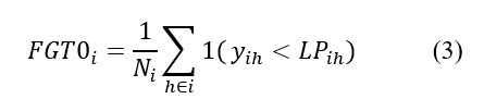
where LP_ih is the poverty line corresponding to the urban or rural domain (Foster et al., 1984). Under the EBP approach, the binary indicator is replaced by its conditional expectation with respect to the posterior distribution of parameters and random effects.
Equation 4

This procedure follows the logic of the Empirical Best Prediction for nonlinear indicators derivable from individual-level models (Molina & Rao, 2010; Rao & Molina, 2015).
Given the normality assumption in the logarithmic scale, the probability of poverty can be derived analytically as:
Equation 5

where Φ(.) is the standard normal cumulative distribution function. Municipal estimation is obtained by aggregating probabilities weighted by the household population weight:
Ecuación 6
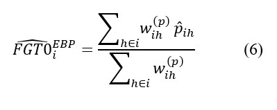
where w_ih^((p) )is the product of the expansion factor and the household size. This aggregation form is consistent with the SAE literature applied to monetary poverty (Lange et al., 2022; Molina & Rao, 2010).
ICAR spatial component: Residual territorial heterogeneity is modeled through an ICAR process:
Equation 7

where W is the municipal neighborhood matrix (Queen) and τ_uis the spatial precision parameter, subject to the constraint ∑_i u_i =0.
The ICAR model derives from the formulation of Gaussian Markov random fields proposed by Besag (1974) and extended in Besag et al. (1991), and constitutes a spatial smoothing mechanism that allows sharing information between contiguous municipalities (Blangiardo & Cameletti, 2015).
Inference and uncertainty propagation: The model is estimated via INLA within the latent Gaussian model framework:
Equation 8
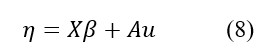
INLA allows deterministic approximation of marginal posterior distributions without resorting to MCMC simulation, being particularly efficient in high-dimensional spatial models (Blangiardo & Cameletti, 2015; Rue et al., 2009).
The ENIGH expansion factors are incorporated as normalized weights in the likelihood, maintaining the model-based interpretation of inference (Rao & Molina, 2015).
To propagate uncertainty toward the municipal indicator, joint posterior replications are generated:
Equation 9

In each replication, the probabilities p ̂_ih^((b) )and the municipal incidence (FGT0) ̂_i^((b) ) are recalculated, thus obtaining the complete posterior distribution of the indicator for each municipality, in accordance with the standard EBP procedure under approximate Bayesian frameworks (Molina & Rao, 2010; Rao & Molina, 2015).
The full model can be summarized as:
Equation 10
 Estimated via INLA with penalized priors complexity (PC priors) for the precision parameters, an approach that allows controlling the effective complexity of the spatial model and avoiding overfitting (Simpson et al., 2017).
Bayesian inference and spatial structure: For estimation of the ALIVIO model, Integrated Nested Laplace Approximation (INLA) is used, a Bayesian inference technique that optimizes computing time in high-dimensional models by employing analytical approximations instead of traditional MCMC simulations (Rue et al., 2009).
Territorial dependence is integrated through an ICAR structure, which assumes that the random component of a municipality is conditioned by its contiguous neighbors. This approach allows borrowing strength from adjacent domains, efficiently capturing residual spatial autocorrelation.
The combination of INLA and ICAR contributes to improving relative precision in latent Gaussian models, enabling agile sensitivity analysis and cross-validations. The result is a statistically robust, territorially coherent national poverty map with explicit uncertainty measures (Blangiardo & Cameletti, 2015).
Results
The posterior mean values of the EBP–ICAR model hyperparameters are:
Equation 11

Most of the residual variability of transformed per capita income is concentrated at the household level, as expected in an individual-level nested error model (Molina & Rao, 2010; Rao & Molina, 2015). Nevertheless, the municipal spatial variance is not negligible.
From these variances, the spatial intraclass correlation coefficient is computed:
Equation 12
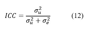
The estimated value (≈ 18%) indicates that approximately one fifth of the residual variability of transformed income is associated with systematic differences between municipalities, after controlling for covariates. This type of decomposition is consistent with the interpretation of random effects in Gaussian hierarchical models (Blangiardo & Cameletti, 2015). The result confirms the empirical relevance of the ICAR spatial component in explaining persistent territorial heterogeneity.
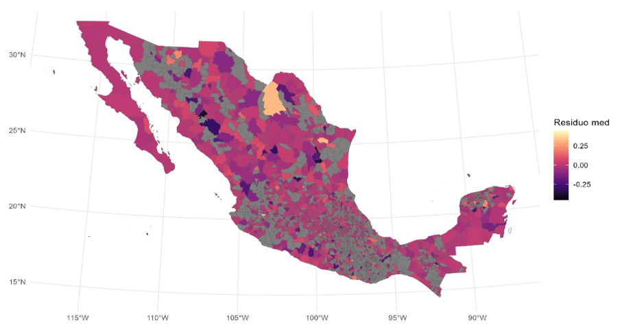
To verify the adequacy of the ICAR component, the presence of residual spatial autocorrelation in aggregate municipal residuals was evaluated. Mean marginal municipal residuals were computed as the weighted average of individual residuals within each municipality (Figure 1).
The spatial pattern shows dispersed residuals, with no formation of large clusters or contiguous regions with persistently high or low values. Most municipalities show residuals close to zero, and the most pronounced deviations appear in isolated fashion.
Overall, these diagnostics indicate that the ICAR spatial effect is identified and centered, that no systematic residual spatial dependence is observed, and that the magnitude of the spatial effect is consistent with the estimated variance decomposition (Figure 1).
Figure 1
Weighted mean municipal residuals of the EBP-ICAR model, Mexico, ENIGH 2024/Census 2020
Source: Own elaboration based on estimates from the ALIVIO model.
Evaluation of the EBP–ICAR model shows better relative performance compared to the direct estimator across the diagnostics considered. The absence of residual autocorrelation validates the spatial specification (Besag et al., 1991), while sensitivity analyses demonstrate that the mean bias remains close to zero regardless of sample size.
In municipalities with at least 30 observations, the correlation between both estimators exceeds 0.90, reflecting the theoretical convergence of the model toward the direct estimate when information is sufficient. However, in domains with small samples, the model introduces a shrinkage effect that reduces the extreme instability of design-based estimators (Chandra et al., 2018; Rao & Molina, 2015).
Comparison of the Relative Root Mean Square Error (RRMSE) shows that the model-based approach offers systematically smaller errors and more stable trajectories. Using smoothed curves (Locally Weighted Regression, LOESS), it is confirmed that the sensitivity of the error to sample size decreases drastically thanks to the borrowing strength of covariates and the spatial structure (Jiang & Rao, 2020). These results suggest that the ALIVIO model provides more stable and territorially coherent estimates even under severe sampling limitations (Figure 2).
Figure 2
Comparison of RRMSE between the direct estimator and the EBP–ICAR estimator for FGT0, by municipal sample size
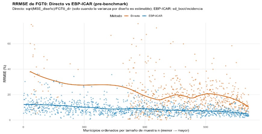
Note. The direct RRMSE is shown only when the design-based variance is estimable (MSE > 0).
Source: Own elaboration based on estimates from the ALIVIO model.
Validation of the EBP–ICAR model confirms its theoretical consistency and statistical robustness. As sample size increases, the estimator converges to the direct estimate; in low-information domains, the model offers a substantial stability gain through the shrinkage effect, reducing extreme variability without introducing systematic biases (Rao & Molina, 2015).
Adequate uncertainty calibration is evidenced by the empirical coverage of intervals, which remains close to nominal levels. Likewise, standardized statistics show decreasing dispersion with respect to sample size, aligning with small area model assumptions (Fay & Herriot, 1979).
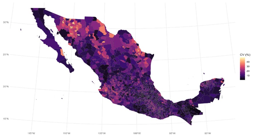
At the national level, precision measured through the coefficient of variation (CV) shows a mean of 13.75%. Notably, more than 97% of municipalities record a CV below 30%, a reference threshold frequently used to evaluate precision in small domains. Spatially, higher precision is concentrated in urban areas, while the highest CVs appear in isolated rural areas, a pattern consistent with the availability of direct information.
Overall, the results show a mean poverty incidence of 49.1% and a median of 48.9%. The absence of systematic low-precision patterns supports the overall stability of the ALIVIO model for generating municipal poverty maps in Mexico, ensuring territorial coherence and formal statistical support (Figure 3).
Figure 3
Coefficient of variation (%) of municipal poverty incidence EBP–ICAR (post-benchmark)
Source: Own elaboration based on estimates from the ALIVIO model.
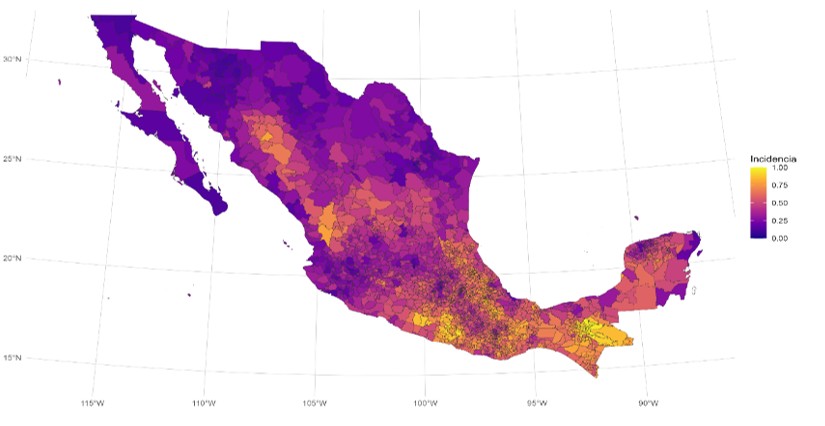
The results reveal marked territorial heterogeneity in Mexico, with incidences ranging from minimum levels in high-income urban centers to values approaching 100% in marginalized rural areas. The geographic pattern identified is fully consistent with the national socioeconomic structure, showing poverty concentrations in the south and southeast, as well as persistence in rural regions of the center and west, contrasting with lower incidence in metropolitan and industrial hubs.
Notably, transitions between municipalities are gradual, evidencing the spatial smoothing effect of the ICAR component (Figure 4). This structure allows capturing territorial dependence and leveraging information from contiguous municipalities without imposing artificial homogenization, ensuring that the map reflects both geographic inertia and local particularities (Blangiardo & Cameletti, 2015).
Figure 4
Municipal poverty incidence — EBP–ICAR (2024 grid)
Source: Own elaboration based on estimates from the ALIVIO model.
Finally, it should be emphasized that the estimates correspond exclusively to monetary poverty measured through the FGT0 index (Foster et al., 1984) and do not replace the official multidimensional measurement; nevertheless, they constitute a valuable input for detailed territorial analysis within a formal statistical framework.
Municipalities with the highest and lowest estimated incidence
To verify the coherence of the model after the state-level adjustment (benchmarking), municipalities with extreme poverty incidences were analyzed, a standard SAE practice for validating inference stability (Rao & Molina, 2015). The ten municipalities with the highest incidence are located in Chiapas, in areas with high marginalization and indigenous populations. These show estimates ranging from 0.949 to 1.000, with extremely low coefficients of variation (below 3%) and narrow credibility intervals.
This high precision and the geographic concentration of results are consistent with the structure of the ICAR model, which leverages information from neighboring municipalities and auxiliary variables to stabilize domains with limited direct data (Molina & Rao, 2010). The alignment of these values with the documented socioeconomic reality supports the robustness and empirical plausibility of the proposed methodology.
Municipalities with the lowest poverty incidence are located in high-income metropolitan areas, such as San Pedro Garza García and boroughs of Mexico City, as well as in nodes with high economic or tourism integration. Estimates in these domains range from 0.012 to 0.105.
In these cases, relatively high coefficients of variation (CV) are observed. This behavior is statistically consistent in SAE: when the mean is very low, the CV tends to increase even if the absolute standard deviation is small (Rao & Molina, 2015). However, the credibility intervals remain bounded, ruling out any structural instability.
In summary, the extreme values generated by the EBP–ICAR model show solid territorial consistency and magnitudes fully compatible with the prevailing socioeconomic evidence, validating the substantive plausibility of the adopted approach (Jiang & Rao, 2020) (Table 2).
Table 2
Municipalities with the highest and lowest estimated incidence — EBP–ICAR (post-benchmark)
Ten municipalities with the highest incidence |
|||||||
State |
Municipality |
Geostatistical locality code |
Incidence |
CV (%) |
SD |
ICr 95% lower |
ICr 95% higher |
Chiapas |
Oxchuc |
07064 |
1.000 |
0.71 |
0.007 |
0.994 |
1.000 |
Chiapas |
Tumbalá |
07100 |
0.994 |
1.21 |
0.012 |
0.965 |
1.000 |
Chiapas |
Tila |
07096 |
0.977 |
1.25 |
0.012 |
0.950 |
0.998 |
Chiapas |
San Juan Cancuc |
07112 |
0.975 |
2.26 |
0.022 |
0.922 |
1.000 |
Chiapas |
Chanal |
07024 |
0.974 |
2.07 |
0.020 |
0.927 |
1.000 |
Chiapas |
Zinacantán |
07111 |
0.967 |
1.37 |
0.013 |
0.937 |
0.989 |
Chiapas |
Pantelhó |
07066 |
0.965 |
2.69 |
0.026 |
0.901 |
1.000 |
Chiapas |
Chilón |
07031 |
0.964 |
0.98 |
0.009 |
0.944 |
0.982 |
Chiapas |
Yajalón |
07109 |
0.963 |
1.43 |
0.014 |
0.933 |
0.986 |
Chiapas |
San Andrés Duraznal |
07118 |
0.949 |
2.62 |
0.025 |
0.891 |
0.989 |
Ten municipalities with the lowest incidence |
|||||||
State |
Municipality |
Location |
Incidence |
CV (%) |
SD |
ICr 95% lower |
ICr 95% higher |
Nuevo León |
San Pedro Garza García |
19019 |
0.012 |
17.9 |
0.002 |
0.008 |
0.017 |
Ciudad de México |
Benito Juárez |
09014 |
0.019 |
7.9 |
0.002 |
0.017 |
0.023 |
Ciudad de México |
Miguel Hidalgo |
09016 |
0.041 |
7.9 |
0.003 |
0.035 |
0.048 |
Nuevo León |
San Nicolás de los Garza |
19046 |
0.085 |
6.5 |
0.006 |
0.075 |
0.097 |
Querétaro |
Corregidora |
22006 |
0.085 |
9.0 |
0.008 |
0.071 |
0.101 |
Sonora |
Huépac |
26034 |
0.090 |
37.2 |
0.034 |
0.041 |
0.171 |
Sonora |
Bacoachi |
26011 |
0.094 |
42.0 |
0.039 |
0.038 |
0.188 |
Baja California |
Playas de Rosarito |
02005 |
0.096 |
12.9 |
0.012 |
0.074 |
0.122 |
Sonora |
Fronteras |
26027 |
0.104 |
28.5 |
0.030 |
0.058 |
0.174 |
Quintana Roo |
Isla Mujeres |
23003 |
0.105 |
22.0 |
0.023 |
0.067 |
0.157 |
Source: Own elaboration based on estimates from the ALIVIO model.
Specification sensitivity analysis
In order to evaluate the robustness of the municipal estimates, the EBP–ICAR model was compared with two alternative specifications, estimated under the same state-level coherence adjustment scheme (benchmarking): a unit-level nested error model without an explicit spatial component (NER–EBP), and a model that incorporates spatial structure through covariates and spatial filters (SLX–ESF).
The NER model constitutes the standard nested error specification used in SAE, where the municipal random effect Ui is assumed to be independently and identically distributed (IID), without incorporating explicit spatial dependence between areas.
For its part, the SLX–ESF specification introduces spatial information through the systematic component of the model. In particular, it incorporates spatial lags of covariates (SLX) and spatial filters based on eigenvectors (ESF), allowing capture of territorial patterns in the linear predictor. However, the municipal random effect remains IID, so spatial dependence is not modeled directly in the random term.
In contrast, the ICAR model explicitly incorporates spatial structure in the municipal random component, assuming that neighboring municipalities exhibit correlated effects. In this way, spatial dependence is modeled as a structured latent process, allowing direct spatial smoothing between contiguous areas.
The objective is not to propose alternative models, but to verify that the main results do not critically depend on a single specification. The comparison between random effect structures and spatial configurations constitutes a standard practice in the validation of spatial hierarchical models (Blangiardo & Cameletti, 2015). Likewise, sensitivity evaluation with respect to the omission of the spatial component allows isolating the specific contribution of the ICAR term to variance reduction and territorial stabilization (Rao & Molina, 2015).
In particular, the comparison between the classical NER model and the version with spatial structure allows identifying the additional smoothing effect induced by explicit territorial dependence, beyond the shrinkage effect already present in the traditional nested error model (Fay & Herriot, 1979; Molina & Rao, 2010).
Comparison between municipal estimates shows a correlation of ρ = 0.593 between ICAR and NER, and ρ = 0.896 between ICAR and SLX–ESF. The high correlation between ICAR and SLX–ESF indicates that both spatial models reproduce similar territorial patterns, while the moderate correlation with NER suggests that the explicit incorporation of spatial structure systematically modifies the territorial distribution, especially in municipalities with sparse sample information. This behavior is consistent with the logic of spatial hierarchical models, where the structured term redistributes information between contiguous domains (Besag, 1974; Blangiardo & Cameletti, 2015).
In absolute terms, the Mean Absolute Error (MAE) is larger between ICAR and NER (0.141 on the proportion scale, equivalent to 14.1 percentage points) than between ICAR and SLX–ESF (0.096 points), confirming that the main divergence occurs between models with and without a spatial component. This difference reflects the additional contribution of territorial smoothing beyond the shrinkage effect of the classical nested error model (Fay & Herriot, 1979; Rao & Molina, 2015).
Comparison of the coefficient of variation (CV) distribution shows a substantial improvement under the ICAR model. The mean CV is reduced from 26.8% in NER to 13.2% in ICAR, while the median moves from 26.0% to 12.1%. More than 82% of municipalities show CV < 20% under ICAR, and only 0.24% exceed the 40% threshold. In addition, the population-weighted mean is considerably lower in ICAR (6.5%), indicating particularly relevant gains in larger municipalities.
In contrast, the NER model shows a concentration in the 25–30% range, while the SLX–ESF exhibits greater dispersion and longer upper tails. The systematic reduction of the CV under ICAR is consistent with SAE theory, where the incorporation of hierarchical structure and spatial dependence allows reducing variance without introducing systematic biases when the model is correctly specified (Newhouse et al., 2022).
The average reduction is 48.7% relative to the NER model, with a median of −53.3% and a 95th percentile of −82.6%. This implies that, in most municipalities, the inclusion of the ICAR spatial effect reduces by approximately half the uncertainty associated with estimation. The magnitude and consistency of this improvement suggest that the spatial effect does not act as a marginal adjustment, but rather as a structural component that increases estimator efficiency in domains with limited information, in line with the principle of leveraging auxiliary informationen SAE (Jiang & Rao, 2020; Rao & Molina, 2015).
The model is estimated under a fully model-based unit-level approach. The ENIGH expansion factors are incorporated as normalized weights in the likelihood to preserve the relative contribution of each observation, without explicitly replicating the complex design (strata and PSUs) as an additional hierarchical structure.
Inference is based exclusively on the posterior distribution obtained via INLA and not on variance approximations derived from the sample design, so results must be interpreted within the model-based framework (Jiang & Rao, 2020; Rao & Molina, 2015). Furthermore, the model already incorporates explicit territorial dependence through the ICAR spatial component. Since PSUs tend to show geographic concentration, simultaneously including intra-PSU and spatial effects could generate overlap in the variance decomposition and identification problems. In spatial hierarchical models, the relevant correlation should be modeled directly in the corresponding random term (Blangiardo & Cameletti, 2015).
In summary, the weights adjust the observational contribution, while territorial dependence is structurally modeled through ICAR, in coherence with the a individual-levelmodel-based (Rao & Molina, 2015).
Discussions
The implementation of the EBP–ICAR model in the ALIVIO project entails a methodological trade-offcharacteristic of model-based approaches: a substantial reduction in variance in exchange for dependence on explicit structural assumptions. In municipal domains with small sample sizes, direct estimators show severe instability and even impossibility of estimation. The incorporation of hierarchical random effects and spatial structure allows redistributing information between domains and stabilizing estimates through shrinkage effect and auxiliary information leveraging mechanisms (Fay & Herriot, 1979; Jiang & Rao, 2020; Rao & Molina, 2015).
Empirical evidence shows a marked reduction in uncertainty and the absence of relevant residual spatial autocorrelation, suggesting that the ICAR component adequately captures the territorial dependence of income (Besag, 1974; Blangiardo & Cameletti, 2015). However, this efficiency gain depends on the validity of the adopted specification and the structural stability of the modeled relationships.
The model combines information from the 2020 Census with the ENIGH 2024, which assumes conditional stability in the relationship between income and covariates. Although this assumption could be compromised by recent macroeconomic changes, the consistency across alternative specifications suggests that results are not dominated by structural instability. Since per capita income exhibits positive skewness and possible zero values, a log transformation with displacement is employed:
Equation 13
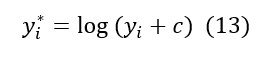
where c> 0 is selected endogenously by minimizing the skewness of the transformed variable. This strategy allows including zero incomes without truncation and reduces the influence of high outliers without resorting to ad hoc procedures. To re-express expected income in the original scale, the smearing estimator of Duan (1983) is used, ensuring consistency in retransformation.
The model depends on covariates harmonized between ENIGH and Census. Although explicit conceptual equivalence criteria were applied, there is always a residual risk of measurement mismatch. However, the stability of territorial patterns and the coherence across spatial specifications suggest that results do not respond to measurement artifacts.
Estimation is carried out entirely on the 2020 municipal grid, consistent with the ICAR spatial structure. The transfer to the 2024 grid via maximum geometric intersection constitutes a cartographic adjustment that does not alter statistical inference or estimated variance, preserving the integrity of the original unit of analysis (Brinegar & Popick, 2010; Gutiérrez et al., 2022).
The estimates depend on official definitions of urban and rural poverty lines and the temporal conversion of income. These thresholds condition classification, so institutional modifications would automatically affect the estimated levels.
Compared to previous exercises, the ALIVIO model explicitly integrates ICAR spatial structure within a individual-level Bayesian framework estimated via INLA (Blangiardo & Cameletti, 2015; Rue et al., 2009). This approach allows capturing persistent territorial heterogeneity and producing complete estimates with formal uncertainty measures.
Although no structural model is exempt from the risk of misspecification, the obtained diagnostics (substantial variance reduction, attenuation of residual spatial dependence, and stability across alternative specifications) suggest that efficiency gains do not generate relevant systematic distortions. Consequently, the proposed approach constitutes a methodologically robust and operationally viable tool for the periodic production of municipal monetary poverty maps, especially in contexts with severe sampling constraints.
Conclusions
This study develops and implements a municipal-level SAE methodology that integrates an EBP-type empirical predictor with an ICAR spatial structure estimated via INLA. The proposed architecture allows coherently combining the ENIGH sample information, the comprehensive Census covariates, and the territorial dependence between municipalities, generating complete estimates for all 2,469 municipalities in the country.
Empirical results show that the incorporation of the spatial component produces a substantial improvement in precision compared to specifications without territorial structure, particularly in municipalities with sparse or zero samples. At the same time, the model maintains global concordance with the direct estimator when sample size is sufficient, reflecting the theoretical shrinkage effect mechanism characteristic of unit-level approaches. The absence of relevant residual spatial autocorrelation and stability across alternative specifications reinforce the empirical validity of the adopted structure.
From an operational perspective, the approach enables generating municipal monetary poverty maps with explicitly quantified uncertainty levels, significantly expanding the analytical capacity available during intercensal periods. This characteristic is especially relevant in contexts where direct representativeness at the municipal level is not feasible through traditional surveys.
In terms of public policy, this granularity allows moving from planning based on state averages to precision targeting (Saeed & Salvati, 2024). By identifying 'poverty pockets' previously hidden by sampling error, authorities can optimize the allocation of budgetary resources and the design of basic social infrastructure programs in municipalities with the greatest monetary lag, contributing to directing intervention toward territories with lower income levels.
Nevertheless, the estimates must be interpreted within the model-based framework adopted. The model depends on assumptions of structural stability between sources, the quality of covariate harmonization, and the official definition of monetary poverty lines. Likewise, the results are confined to income poverty and do not replace the official multidimensional measurement.
Substantively, the findings confirm that poverty in Mexico is not an isolated municipal phenomenon but exhibits strong territorial inertia; that is, the probability of being poor is conditioned not only by household characteristics but by the socioeconomic performance of neighboring municipalities. This interpretation suggests that poverty reduction strategies must adopt a coordinated regional approach, breaking the logic of isolated municipal action.
Beyond statistical efficiency, the results of the ALIVIO model offer a substantive interpretation of the configuration of poverty in Mexico: it is not distributed randomly, but exhibits a territorial inertia where the vulnerability of a municipality is intrinsically linked to the performance of its regional environment.
The identification of 'poverty pockets' and critical clusters, previously rendered invisible by sampling error in traditional surveys, provides decision-makers with a roadmap for optimizing budget allocation. By reducing uncertainty in municipalities with 'zero sample', the ALIVIO approach ensures that investment in social infrastructure and transfer programs can be directed with greater accuracy to territories where income deprivation is structural, promoting distributive justice based on granular statistical evidence.
In methodological terms, the project contributes to the applied literature in Latin America (Gutiérrez et al., 2024) by explicitly incorporating ICAR spatial structure within a unit-level framework replicable with official data. To ensure the replicability of the approach, the importance of maintaining a harmonized variable dictionary between the Census and the ENIGH is emphasized, as well as the use of open-source libraries for INLA implementation, allowing local statistical institutions to systematically adopt the model.
It must be acknowledged that the rigor of these estimates is conditioned on the validity of the model-based framework. First, precision critically depends on structural stability and the quality of harmonization between the ENIGH and the Census. Second, the approach assumes normality and linearity assumptions that must be monitored in the face of abrupt changes in income distribution. Finally, although ALIVIO successfully resolves monetary poverty estimation, this is only one dimension of well-being; results should be considered complementary to, not substitutes for, the official multidimensional measurement. As a future agenda, the extension toward spatio-temporal structures that allow evaluating the dynamism of these indicators in the face of economic shocks remains pending.
Future research lines include: (i) extending the model toward spatio-temporal structures that capture the evolution of income gaps in the face of macroeconomic shocks, (ii) exploring alternative neighborhood schemes that incorporate economic connectivity and labor commuting flows, and (iii) deepening external validation strategies through the use of non-conventional data sources (big data or satellite imagery) in zero-sample domains.
Overall, the ALIVIO approach offers a robust technical foundation for strengthening the production of territorial evidence in Mexico. By overcoming the fragmentation of municipal data, it facilitates an inequality analysis that recognizes the continuity of the social and economic fabric, supporting public planning processes based on statistically consistent and spatially coherent information.
Ethical considerations
This research did not require ethical approval as it was based on documents from government institutions.
Conflict of interest
All authors made significant contributions to the document and declare that no there is no conflict of interest related to this article.
Statement of contribution of the authors
Víctor Adrián Morales Linares: conceptualization, methodology, formal analysis, data curation, writing-original draft.
Beatriz Martínez Carreño: validation, writing: review and editing, supervision, project administration, writing-original draft
María Isabel Garrido Lastra: conceptualization, investigation, writing-original draft, writing: review and editing.
Source of funding
The article has no funding sources.
References
(1)Arias, A. (2023). Small area estimates of poverty incidence in Costa Rica under a Structure Preserving Estimation (SPREE) approach. Journal of Official Statistics, 39(4), 435–458. https://doi.org/10.2478/jos-2023-0021
(2)Arima, S., Datta, G. S. & Liseo, B. (2015). Bayesian estimators for small area models when auxiliary information is measured with error. Scandinavian Journal of Statistics, 42(2), 518–529. https://doi.org/10.1111/sjos.12120
(3)Ballini, F., Betti, G., Carrette, S. & Neri, L. (2006). Mapeo de la pobreza y la desigualdad en la Mancomunidad de Dominica. Estudios Económicos, 2, 123–162. https://doi.org/10.24201/ee.v0i0.384
(4)Besag, J. (1974). Spatial interaction and the statistical analysis of lattice systems. Journal of the Royal Statistical Society: Series B (Methodological), 36(2), 192–236. https://doi.org/10.1111/j.2517-6161.1974.tb00999.x
(5)Besag, J., York, J. & Mollié, A. (1991). Bayesian image restoration, with two applications in spatial statistics. Annals of the Institute of Statistical Mathematics, 43(1), 1–20. https://doi.org/10.1007/BF00116466
(6)Blangiardo, M. & Cameletti, M. (2015). Spatial and spatio-temporal Bayesian models with R-INLA. John Wiley & Sons. https://doi.org/10.1002/9781118950203
(7)Brinegar, S. J. & Popick, S. J. (2010). A comparative analysis of small area population estimation methods. Cartography and Geographic Information Science, 37(4), 273–284. https://doi.org/10.1559/152304010793454327
(8)Cameletti, M., Finazzi, F. & Lindgren, F. (2013). Spatio-temporal integrated nested Laplace approximation for disease mapping. Advances in Statistical Analysis, 97(2), 241–261. https://doi.org/10.1007/s10182-012-0196-3
(9)Chandra, H., Salvati, N. & Chambers, R. (2018). Small area estimation under a spatially non-linear model. Computational Statistics & Data Analysis, 126, 19–38. https://doi.org/10.1016/j.csda.2018.04.002
(10)Comisión Económica para América Latina y el Caribe (CEPAL). (2025). Definición de ingreso corriente per cápita. Naciones Unidas. https://www.cepal.org/es
(11)Consejo Nacional de Evaluación de la Política de Desarrollo Social (CONEVAL). (2020). Metodología para la medición multidimensional de la pobreza en México (3.ª ed.). CONEVAL. https://www.coneval.org.mx/InformesPublicaciones/InformesPublicaciones/Documents/Metodologia-medicion-multidimensional-3ed.pdf
(12)Duan, N. (1983). Smearing estimate: A nonparametric retransformation method. Journal of the American Statistical Association, 78(383), 605–610. https://doi.org/10.1080/01621459.1983.10478017
(13)Fay, R. E. & Herriot, R. A. (1979). Estimates of income for small places: An application of James-Stein procedures to census data. Journal of the American Statistical Association, 74(366a), 269–277. https://doi.org/10.1080/01621459.1979.10482505
(14)Foster, J., Greer, J. & Thorbecke, E. (1984). A class of decomposable poverty measures. Econometrica, 52(3), 761–766. https://doi.org/10.2307/1913475
(15)Gutiérrez, A., Mancero, X. & Guerrero, S. (2022). Poverty mapping in Latin America. Statistical Journal of the IAOS, 38(3), 1021–1033. https://doi.org/10.3233/SJI-220037
(16)Gutiérrez, A., Mancero, X. & Trujillo, L. (2024). Poverty mapping in Latin America using advanced small area estimation models. Journal of Official Statistics, 40(3), 615–639. https://doi.org/10.3233/SJI-220037
(17)INEGI. (2024). Encuesta Nacional de Ingresos y Gastos de los Hogares (ENIGH) 2024. INEGI. https://www.inegi.org.mx/programas/enigh/nc/2024/
(18)Instituto Nacional de Estadística y Geografía (INEGI). (2020). Censo de Población y Vivienda 2020. INEGI. https://www.inegi.org.mx/programas/ccpv/2020/
(19)Jiang, J. & Rao, J. N. (2020). Small area estimation. John Wiley & Sons. https://doi.org/10.1002/9781118445112.stat03310.pub2
(20)Lange, S., Pape, U. J. & Pütz, P. (2022). Small area estimation of poverty under structural change. Review of Income and Wealth, 68(S2), S264–S281. https://doi.org/10.1111/roiw.12558
(21)Marchetti, S., Giusti, C., Schirripa, F., Bertarelli, G. & Biggeri, L. (2024). The impact of local cost‑of‑living differences on relative poverty incidence: An application using retail scanner data and small area estimation models. Statistical Methods & Applications, 33(4), 1117–1143. https://doi.org/10.1007/s10260-023-00742-w
(22)Molina, I. & Rao, J. N. K. (2010). Small area estimation of poverty indicators. Canadian Journal of Statistics, 38(3), 369–385. https://doi.org/10.1002/cjs.10051
(23)Molina, I. (2024). Frontiers in small area estimation research: Application to welfare indicators (Policy Research Working Paper No. 10828). World Bank. https://doi.org/10.1596/41801
(24)Morales, D., Esteban, M. D., Pérez, A. & Hobza, T. (2021). A course on small area estimation and mixed models. Springer. https://doi.org/10.1007/978-3-030-63757-6
(25)Mweemba, C., Hangoma, P. & Masiye, F. (2022). Estimating district HIV prevalence using SAE. Population Health Metrics, 20(1), 22. https://doi.org/10.1186/s12963-022-00286-3
(26)Newhouse, D., Ramakrishnan, A., Swartz, T., Merfeld, J. & Lahiri, P. (2022). Small area estimation of monetary poverty in Mexico using satellite imagery (Policy Research Working Paper N.º 10123). Banco Mundial. https://doi.org/10.1111/obes.12678
(27)Possolo, A. (2023). Tracking truth through measurement and the spyglass of statistics. Statistical Science, 38(4), 655–671. https://doi.org/10.1214/23-STS899
(28)Purwa, T., Rumiati, A. T. & Zain, I. N. (2019). Small area estimation with bivariate hierarchical Bayes (HB) approach to estimate monthly average per capita expenditure of food and non-food commodities in Province of Bali. IOP Conference Series: Materials Science and Engineering, 546(5), 052054. https://doi.org/10.1088/1757-899X/546/5/052054
(29)Rao, J. N. K. & Molina, I. (2015). Small area estimation (2.ª ed.). John Wiley & Sons. https://doi.org/10.1002/9781118735855
(30)Rue, H., Martino, S. & Chopin, N. (2009). Approximate Bayesian inference for latent Gaussian models by using integrated nested Laplace approximations. Journal of the Royal Statistical Society: Series B (Statistical Methodology), 71(2), 319–392. https://doi.org/10.1111/j.1467-9868.2008.00700.x
(31)Saeed, M. & Salvati, N. (2024). Spatial autocorrelation and business-cycle effects on regional poverty mapping. Spatial Economic Analysis, 19(2), 201–224. https://doi.org/10.3390/ijgi12120501
(32) Simpson, D. P., Rue, H., Riebler, A., Martins, T. G. & Sørbye, S. H. (2017). Penalising model component complexity: A principled, practical approach to constructing priors. Statistical Science, 32(1), 1–28. https://doi.org/10.1214/16-STS576